Simetar© consists of both Menu Driven Functions and User Defined Functions that run in Excel. A common theme with Simetar©, is that all functions are dynamic; so if changes are made to the original data most all parameters, hypothesis tests, regression models, and risk ranking strategies are automatically updated. This feature of having Excel dynamically recalculate parameters offers significant efficiencies during the development, validation and verification steps for developing stochastic simulation models. The more than 250 User Defined functions in Simetar© can be categorized into six groups: (1) simulating random variables, (2) statistical analyses and tests, (3) graphical analysis, (4) ranking risky alternatives, (5) data manipulation and analysis, (6) econometric modeling, and (7) forecasting.
Simulating a stochastic model in Excel is accomplished by drawing random values for each of the random variables, letting Excel calculate the model’s equations, and save the results of key output variables (KOV) for future analysis. Repeating this process a large number of times (iterations) causes the model to be simulated for a wide range of possible combinations of the random variables. The resulting array of 100 or more simulated values for a KOV define an empirical probability distribution for the output variable. Probability distributions for the output variables are analyzed to gain a better understanding of their range of possible outcomes. Sensitivity tests on key input variables and scenario analysis for management control variables are capabilities required for a complete simulation modeling package. Simetar© provides easy to use tools for simulating a stochastic model, as well as conducting sensitivity tests, analyzing multiple scenarios, and ranking risky alternatives.
Simetar© provides functions for generating pseudo-random numbers from more than 40 probability distributions. A quick guide to simulating random numbers in Excel with Simetar© is provided here. A detailed description of each Simetar© function for simulating random numbers is provided in Section 3 of the User’s Manual. See the Probability Distributions_XLS workbook for examples of how these functions are used in Excel.
| • Uniform distribution • Normal distribution • Discrete Uniform • Truncated Normal • Empirical distribution • Truncated Empirical• Discrete Empirical • GRK distribution • GRKS distribution • Triangle distribution • Bernoulli distribution • Binomial distribution • Negative Binomial • Pareto distribution • PERT distribution • Poisson distribution • Geometric distribution • Hypergeometric distribution • Weibull distribution • Cauchy distribution • Extreme Value distribution • Exponential distribution • Double Exponential distribution • Random sampling with replacement • Correlated standard normal deviates • Correlated uniform standard deviates • Wishart distribution • Hotelling T-Squared distribution • Wilks Lamda distribution • Cosin distribution • Inverse gaussian distribution • Logistic distribution • Log-log or Gumbel distribution • Log-logistic distribution • Modified two-piece normal distribution • Multinomial distribution • Multivariate empirical distribution • Multivariate normal distribution • Power normal distribution • Semicircle distribution • Two-piece normal distribution |
=UNIFORM(min, max) =NORM(mean, std dev) =RANDSORT(array of sorted values) =TNORM(mean, std dev, [min], [max]) =EMPIRICAL(sorted values, F(x) sorted values) =TEMPIRICAL(sorted values, F(x) sorted values, min value, max value, USD) =DEMPIRICAL(array of sorted values) =GRK(min, middle, max) =GRKS(min, middle, max) =TRIANGLE(min, mode, max) =BERNOULLI(probability of a true outcome) =BINOMINV(no. trials, prob of success, USD) =NEGBINOMINV(no. failures, prob of success, USD) =PARETO(alph, beta, USD) =PERTINV(a, b, c, USD) =POISSONINV(l, USD) =GEOMINV(probability of each trial, USD) =HYPERGEOMINV(n,m,k,USD) =WEIBINV(alpha, beta, USD) =CAUCHY(median, sigma, USD) =EXTVALINV(X, mu, sigma, USD) =EXPONINV(beta, USD) =DEXPONINV(mu, sigma, USD) =BOOTSTRAPPER(array of sorted values) =CSND(correlation matrix) =CUSD(correlation matrix) =WISHINV(c, df) =HOTELLINV(p, df, [USD]) =WILKLINV(p, N1, N2) =COSINV(center, radius, USD, max iter, precision) =INVGAUS(mu, sigma, USD, max iter, precision) =LOGISTICINV(mu, sigma, USD) =LOGLOGINV(mu, sigma, USD) =LOGLOGISTICINV(alpha, beta, USD) =MTPNORM(min, middle, max, USD, lower SD, upper SD) =MULTINOMINV(no. of trials, vector probabilities, USD) =MVEMPIRICAL(matrix of values) =MVNORM(vector of means, covariance matrix) =PNORM(mu, sigma, exponent p, USD) =SEMICIRCINV(center, radius, USD, maxiter, precision) =TPNORM(mu, std dev lower, std dev upper, USD) |
|
The following probability distributions provided by Excel, can be simulated with Simetar© if the USD is a uniform standard deviate generated using Simetar’s uniform distribution function = UNIFORM().
| • Beta distribution • Chi-Squared distribution • Gamma distribution • Log Normal distribution • Student’s t distribution • F distribution |
=BETAINV(USD, alpha, beta, min, max) =CHIINV(USD, mean) =GAMMINV(USD, alpha, beta) =LOGINV(USD, mean, std dev) =TINV(USD, degrees of freedom) =FINV(USD, degree of freedom1, degree of freedom2) |
|
Simetar© offers users an option to select their random number generator. Four random number generators are available: Excel’s Native generator, the Mersine Twister, the L’Ecuyer’s Combined Multiplicative Random Number Generator, and the native generator in Microsoft Visual C++. For each random number generator, the user may select to sample random numbers as Latin hypercube or Monte Carlo and the user may specify their own seed.
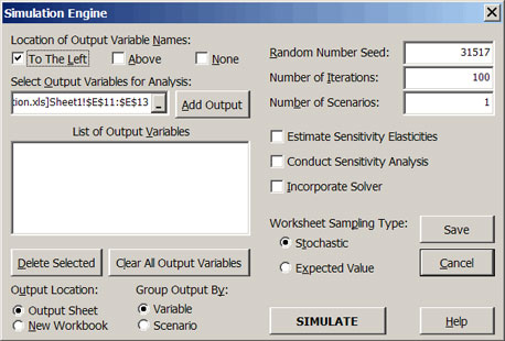
The dialog box for simulating a stochastic Excel simulation model shown in Figure 1 is accessed by the icon
Simulation options for simulating and Excel workbook on the toolbar. Options specified in the dialog box are saved by selecting the Save or the SIMULATE buttons.
 Simulation options for simulating and Excel workbook
 |
| Figure 1. Simulation Dialog Box for Simetar©. |
The user must define one or more key output variables (KOVs) for Simetar© to calculate statistics after simulating the model. Specify the Location of the Output Variable Name by clicking, Left, Above or None, prior to clicking on the Add Output button. The title can be either in the cell to the left and/or above the KOV cell. Add variables to the List of Output Variables box by clicking in the Select Output Variables box, highlighting the cell or cells to include, and clicking the Add Output box. Several hundred output variables can be handled by Simetar©. The sample menu in Figure 1 shows that the variables in E11-E13 are the output variables. To delete an output variable or several variables, highlight the variables in the dialog box and click the Delete Selected button. Clicking on the Clear All Output Variables button will delete all of the output variables listed in the dialog box. Clicking on an output variable in the List of Output Variables box causes Excel to highlight the particular variable in the workbook.
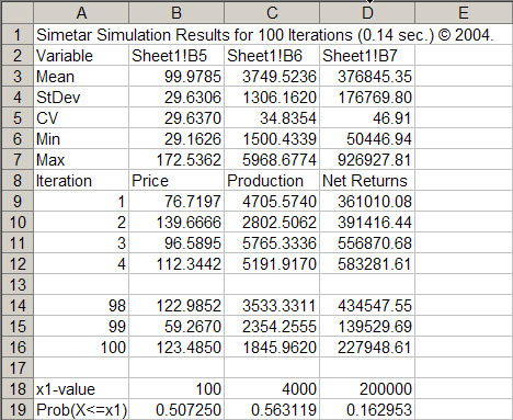
After specifying the output variable(s) click the SIMULATE button and Simetar© will simulate the workbook and save the simulated values for the output variables in a worksheet named SimData. The statistics for each output variable are provided in rows 3-7 of SimData and the simulated values for each variable, by iteration, start in row 9 (Figure 2). Following the simulated data are 10 rows of pre-programmed equations to calculate the probability of the output variable being less than a specified target. Type in a target value in a row labeled “ ” and the probability of the variable being less than or equal to the value will appear in the next row labeled “Prob .” For example, there is a 16.295 percent chance that net returns will be less than $200,000 (see the last column of Figure 2).
The simulated variables in the SimData worksheet always appear in the order they were added to the List of Output Variables (Figure 1). The rows of simulated values for the output variables correspond to the actual iterations as they were simulated, i.e., the iteration order is maintained across output variables in SimData. The simulated values of each iteration for all output variables are provided so the user can analyze the results using Simetar© functions, (such as: hypothesis tests and stochastic efficiency) and different types of charts for presenting risky results.
 |
| Figure 2. Example of Stochastic Results from Simetar©. |
