Functions to facilitate analysis of seasonal and cyclical data are included in Simetar©. Cyclical indices and moving average analysis of cyclical data are described in this section. Three different procedures for developing exponential forecasts included in Simetar© are described in this section as well.
Cyclical Index
A cyclical index of any array can be calculated by Simetar© using the Forecasting and Cyclical Data icon Forecasting with exponential smoothing and seasonal indices and clicking on the Cyclical Indexing tab. The Cyclical Indexing dialog box (Figure 1) allows the user to specify the data series to analyze and the number of periods in the cycle, (say, 4 or 8 or 12).
 Forecasting with exponential smoothing and seasonal indices
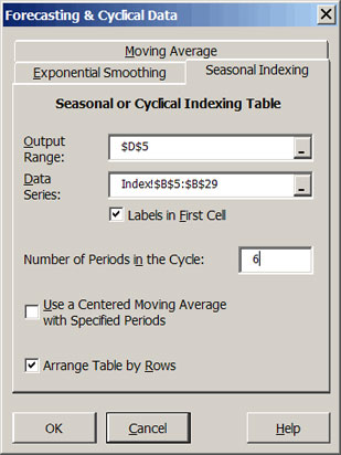 |
| Figure 1. Cyclical Indexing Dialog Box. |
When the input data are months and the Number of Periods in the Cycle is 12 the result will be a 12 month seasonal index. See the Indices worksheet in DemoSimetar-Cycle for an example of a 12 month seasonal price index developed from 36 years of monthly data. The six period index in Figure 2 was developed from 36 annual average prices, to test for a six year cycle.
A seasonal index can be calculated one of two ways, namely: simple average or centered moving average. The simple average index is a more reliable indicator of the seasonal pattern if the data has no trend. If the data series has an underlying trend the centered moving average will remove a portion of the variability caused by the trend. The Cyclical Indexing dialog box (Figure 1) assumes the user wants a simple average index. Click on the Use a Centered Moving Average with Specified Periods option and specify the number of periods to calculate a centered moving average index.
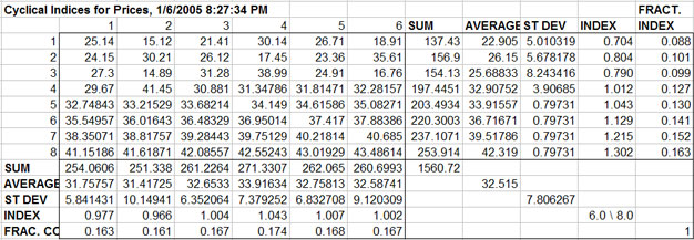 |
| Figure 2. Sample Cyclical Index Output Table. |
Moving Average Forecast
A moving average of any series can be calculated by selecting the forecasting icon Forecasting with exponential smoothing and seasonal indices and selecting the Moving Average tab (Figure 3). The Moving Average dialog box requires information on the number of periods to include in the moving average and the number of periods to forecast.
 Forecasting with exponential smoothing and seasonal indices
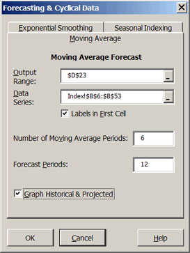 |
| Figure 3. Moving Average Forecast Dialog Box. |
Once Simetar© has completed the analysis you can interactively change the number of periods for the moving average in the output table to observe how that affects the goodness of fit measures. The MAPE, RMSE, and MAE are included in the output so you can experiment with different moving average lengths and observe their affects on these measures of forecast error. A graph of the historical and predicted values is provided as well. See the Moving Average worksheet in DemoSimetar-Cycle for an example.
Exponential Smoothing Forecast
An exponential smoothing forecast for any data series can be developed using the forecasting icon Forecasting with exponential smoothing and seasonal indices and selecting the Exponential Smoothing tab (Figure 4). Simetar© provides three different exponential smoothing estimator/forecasts tools:
 Forecasting with exponential smoothing and seasonal indices
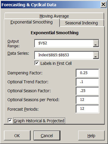 |
| Figure 4. Exponential Smoothing Forecast Dialog Box. |
| • | Single exponential smoothing estimates one parameter alpha (Dampening Factor). |
| • | Double exponential smoothing or Holt’s method estimates parameters for two parameters alpha and beta (Optional Trend Factor). |
| • | Triple exponential smoothing or Holt-Winter’s method estimates three parameters alpha, beta, and gamma (Optional Seasonal Factor). |
Simetar© estimates and forecasts the appropriate model based on the non-zero initial guesses the user provides in the dialog box (Figure 4).
After Simetar© estimates the initial model, you can experiment with alternative parameters to see what they do to the MAPE, RMSE, and MAE. If you specified Holt or Holt-Winter’s exponential smoothing procedures, you must use Excel’s Solver to estimate the parameters which minimize the MAPE. To use Solver select Tools > Solver … on the toolbar and specify the MAPE as the Target Value, the parameters (alpha, beta, and gamma) as the Change Variables, and impose constraints that the parameters must be between zero and one. See the Exponential Smoothing worksheet in DemoSimetar-Cycle for an example.
Measuring Forecast Errors.
Three functions are included in Simetar© for quantifying forecast errors. The functions are found in most statistics books so the equations are not presented here.
• Mean Absolute Percent Error function is: =MAPE (array of residuals, array of history)
• Mean Absolute Error function is: =MAE (array of residuals)
• Root Mean Square Error function is: =RMSE (array of residuals)
where: Array of Residuals is the cell reference for the array of errors or residuals, and
Array of History is the cell reference for the array of historical data that was used to generate the residuals.
Examples of these functions are demonstrated in DemoSimetar-Cycle on the Exponential Smoothing worksheet. Also, the =MAPE( ) function is demonstrated in all of the DemoForecast workbooks.
Simetar© functions for estimating time series models are included in this section. Functions that can be used to test for stationarity are described first, followed by a general autoregressive model menu for estimating autoregressive (AR) and vector autoregressive (VAR) models. The time series analysis functions facilitate parameter estimation and forecasting with both AR and VAR models to aid in developing probabilistic forecasts for simulation. The time series capabilities of Simetar© are demonstrated in DemoSimear-Ar.
Tests for Stationarity
Time series models should only be estimated for series that are stationary. A series can generally be made stationary by differencing. An accepted test for determining if a series is stationary is the Dickey-Fuller test.
The Dickey-Fuller Test can be calculated using a Simetar© function =DF ( ). The =DF( ) function allows the user to test for alternative combinations of differences in an efficient manner to find the combination of adjustments necessary to make a series stationary. Several examples of using the =DF( ) function are provided below to demonstrate how it can be used. The basic Dickey-Fuller Test is coded as:
=DF(Y Values Range)
The Augmented Dickey-Fuller Test that includes a trend is:
=DF(Y Values Range, 1)
The Augmented Dickey-Fuller Test that has no trend and tests for the presence of a second order autocorrelation lag is:
=DF(Y Values Range, 0, 2)
The Augmented Dickey-Fuller Test that includes trend and tests for the presence of a second order autocorrelation lag is:
=DF(Y Values Range, 1, 2)
The null hypothesis for the Dickey-Fuller Tests is: H0: Data Series is nonstationary. The critical test statistic for the Dickey-Fuller Test, based on large sample theory, is approximately -2.9 at the 5% level. The null hypothesis is rejected if the DF statistic is less than the -2.9 critical value. In other words, the series is considered to be stationary if the DF statistic returned by Simetar© is less than -2.9. The Dickey-Fuller test is demonstrated in Step 1 of the Tests worksheet in DemoSimetar-Ar and in Figure 5. The Dickey-Fuller tests for the Wichita data are reported for alternative lags and differences show how the function can help identify the combination of differences, trend, and lags necessary to make the raw data series stationary.
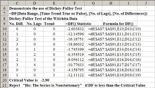 |
| Figure 5. Table for Calculating the Number of Differences for an AR Model. |
Number of Lags
In time series analysis it is essential to determine the optimal number of lags for the AR model after determining the number of differences to make the series stationary. The =ARLAG() function in Simetar© suggests the optimal number of lags to use for the AR model. The =ARLAG( ) function returns the number of lags that minimizes the Schwarz criterion given a particular number of differences. The function is programmed as:
=ARLAG (Y Values Range, [Optional Constant], [Optional No. of Diff])
where: Y Values Range is the range of the time series data to be evaluated, Optional Constant is an optional term if the AR model is expected to have a constant term (true or 1) or has no constant (false or 0). The default is to use a constant term (true) if the value is omitted, and
Optional No. of Diff is the number of differences of the original data series Y assumed to make the series stationary.
The =ARLAG( ) function bases its suggestion of the number of lags on the Schwarz criterion test. The test statistic for the Schwarz criterion is calculated by the following Simetar© function
=ARSCHWARZ (Y Values Range, [Optional Constant], [Optional No. of Diff])
where: All parameters are defined the same as the ARLAG function.
A table for implementing the =ARLAG( ) and =ARSCHWARZ( ) functions is demonstrated in Figure 6. In Excel these functions are dynamic so you can change the number of differences or the presence of a constant and observe the change in the test statistics. An example of how the =ARLAG( ) and the =ARSCHWARZ( ) functions are used is provided in the Tests worksheet of DemoSimetar-Ar. Both tests are demonstrated in Step 2 for 1-6 differences, with and without the constant term. Use the =ARSCHWARZ( ) function to test alternative differences; select the lag structure that minimizes the Schwarz test statistic.
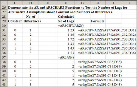 |
| Figure 6. Table for Testing the Optimal Number of Lags in an AR Model. |
Sample Autocorrelation Coefficients
In time series modeling it is useful to estimate the sample autocorrelation coefficients and the sample partial autocorrelation coefficients. These coefficients are calculated using the Simetar© functions =AUTOCORR( ) and =PAUTOCORR( ). The functions are programmed as:
=AUTOCORR (Y Values Range, No. of Lags, No. of Diff) and
=PAUTOCORR (Y Values Range, No. of Lags, No. of Diff)
where: Y Values Range is the range of the time series data to be evaluated, No. of Lags is the number of higher order lags to test, and No. of Diff is the number of differences of the original data series Y to test.
Both of these functions can be used as “scalar” or “array” functions. When used as a scalar, the functions return a single value in the cell which is highlighted. The value returned is the correlation coefficient or the partial autocorrelation coefficient. To use these functions in their array form, highlight three cells in a 3×1 or 1×3 pattern, enter the function name and parameters indicated above, and then press the Control Shift Enter keys. Three values will be calculated and placed in the highlighted array. The first value (top or left most) is the autocorrelation or partial autocorrelation coefficient. The next (middle) value is the Student-t statistic for the coefficient. The last value is the standard error for the coefficient. In the array form these functions can be used to develop tables showing the autocorrelation coefficients and their levels of statistical significance for alternative numbers of lags and differences. An example of using the two functions to estimate sample autocorrelation and partial autocorrelation coefficients is provided in Figure 7 and the Tests worksheet of the DemoSimetar-Ar workbook. Four different lags and first and second differences were tested for the Wichita data series in Step 3. Both autocorrelation functions are demonstrated in array form and the partial autocorrelation coefficient function is demonstrated as a scaler to develop a table of test statistics.
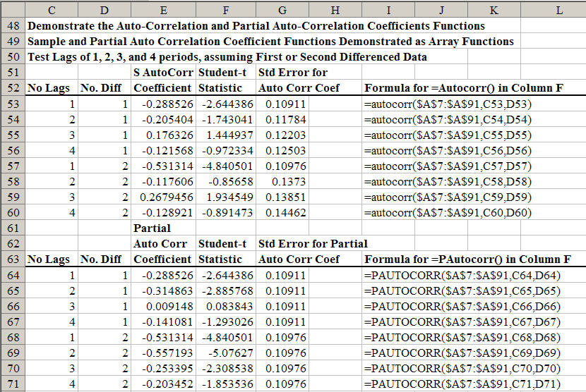 |
| Figure 7. Table for Testing the Autocorrelation and Partial Correlation Coefficients. |
Maximum Likelihood Ratio Test
A maximum likelihood ratio test (LRT) is included as a function in Simetar© to facilitate estimation of the number of lags for an unrestricted vector autoregressive (VAR) model. The LRT is estimated for alternative possible lags using the following function:
=LRT (Y Values Range, No. of Lags, Constant, No. of Diff, Error Correction)
where: Y Values Range is the range of the time series data to be evaluated for potential inclusion in a VAR. Two or more data series must be identified.
No. of Lags is the number of lags to test,
Constant is a switch as to whether a constant term (True or 1) is to be included or not (False or 0),
No. of Diff is the number of differences of the original data series to test, and
Error Correction is whether to perform an error correction (True or 1) on the data or not (False or 0). The =LRT( ) is demonstrated in the Tests worksheet of the DemoSimetar-Ar workbook as Step 4. Two data series were tested for 7 different lags assuming first difference, a constant, and no error correction. The parameters for the =LRT( ) are displayed in a table below the LRTs so one can easily change a parameter and observe the changes in the LRTs.
Estimating and Forecasting Autoregressive Models
The Time Series Analysis Engine menu (Figure 8) provides the mechanism to program the information necessary to estimate and forecast an auto-regressive (AR) model. The Time Series Analysis Engine is activated by selecting the icon. If you specify the data to analyze as a single variable (column of data) in the Data Series window, the Time Series Analyzer will estimate an AR model. (Specifying two or more columns causes Simetar© to estimate a VAR model.) The Number of Lags and Number of Differences for the original data must be specified for the AR model. In addition, provisions are available in the dialog box to indicate whether or not the Constant is Zero. The number of Forecast Periods to project using the estimated model is also specified in the dialog box. It is recommended that the Time Series Engine be programmed to: (a) calculate the residuals, (b) graph the historical and projected values, and (c) graph the impulse response function (Figure 8).
 AR and VAR time series model estimates
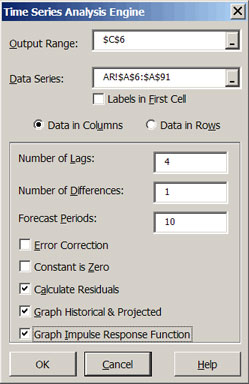 |
| Figure 8. Time Series Analysis Dialog Box. |
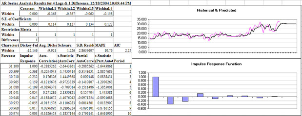
The results of estimating an AR model with four lags and one difference or an AR (4,1) model is presented in the AR worksheet of the DemoSimetar-Ar workbook. Several supporting tests are provided along with the coefficients, namely, the Schwarz test, and two Dickey-Fuller tests. The forecast values for the AR model are provided for 10 periods, as programmed in the dialog box, and are labeled “Forecast.” “Impulse Response” values are provided for each forecast period (Figure 9). Student-t statistics for the sample and partial autocorrelation coefficients are provided for the 10 periods of forecast output.
 |
| Figure 9. Results of Estimating an Autoregressive Time Series Model. |
The time series output generated by Simetar© is dynamic meaning that the beta coefficients in the AR model will update if you change the values in the original data or replace the input data array with another series of data. An added feature is the capability to impose restrictions on the initial AR model by dropping out/re-entering lags on the fly. The Restriction Matrix has 1’s beneath each lags’ (variables’) coefficient. When the restriction value of 1 is changed to 0 the model is re-estimated without that particular variable or lag. The example AR model in DemoSimetar-Ar was run with 4 lags so the user can experiment with deleting unnecessary lags using the Restriction Matrix. When the 2nd, 3rd and 4th lags are restricted out the standard deviation for the residuals increases slightly from 2.86 to 3.06. As these higher order lags are removed the MAPE increases only about 1.3 percentage points.
Note that the initial number of lags and differences specified for the AR model determines the number of observations used to estimate the coefficients. When an AR model of 1st differenced data is estimated with four lags initially but the 3rd and 4th lags are restricted out, the resulting coefficients will not equal those for an AR(1) model estimated with two lags. The reason the coefficients are slightly different is that the latter model uses two more observations to estimate the parameters. It is recommended that the restricted AR model be re-estimated using the exact number of lags once the restricted model is acceptable.
As the restrictions on the lags are imposed on the unrestricted model the following test statistics do not change: Dickey-Fuller Test, Augmented Dickey-Fuller Test, and Schwarz Test (Figure 9). These statistics do not change because they reflect the number of differences specified for the unrestricted model. For example, the Dickey-Fuller Test statistic for an AR(4,1) model is calculated as =DF(data,,,1) and for an AR(4,2) model it is =DF(data,,,2). The Schwarz Test statistic is based on the number of differences [=ARSCHWARZ(data,,No. of Differences)] and does not change as the number of lags is restricted.
It is possible to interactively analyze the impact of changing the number of differences to the data in the AR model. In the second row of the Restriction Matrix (Figure 9) is the word Differences followed by a value, in this case 1. The 1 in the Difference row means the data have been differenced once. To “re-run” the model with second differenced data type a 2 into the restriction matrix in place of the 1. This change causes Simetar© to re-estimate all of the parameters and update the goodness of fit test statistics.
The predicted values over the historical period and their residuals are provided for the AR model. The residuals are also expressed as a fraction of the predicted data. The predicted values and the residuals begin with observation 6, for this example, because the lag/difference structure of an AR(4,1) model uses the first 5 observations.
A graph of the historical and predicted values for the data series is generated by the Time Series Engine. The thin line represents the original data while the bold line represents the predicted values. Projections beyond the historical data in the graph correspond to the 10 period forecast requested in the dialog box (Figure 9).
A graph of the Impulse Response Function is also included in the forecast. The impulse response values are included in the output, but they are easier to see in the graph. A stationary model will exhibit continuously decreasing impulse responses to a 1 unit change at the outset of the period, as depicted by the graph in the AR Worksheet. The Impulse Response Function graph changes as the lags in the model are restricted out. Not shown in Figure 9 is the autocorrelation and partial autocorrelation function graphs for the AR model.
Estimating and Forecasting Vector Autoregressive (VAR) Models
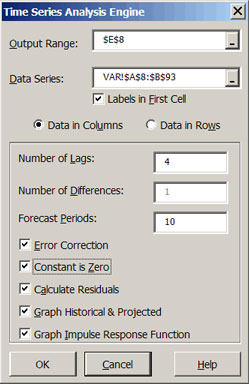
The Time Series Analysis Engine dialog box (Figure 8) can be used to estimate and forecast unrestricted VAR models. VAR model analyses begin by selecting the icon on the Simetar© toolbar. To estimate a VAR model, take all the steps used to estimate an AR model with one exception, specify two or more adjacent series in the Data Series window (Figure 10). When two or more data series are specified, Simetar© uses the more general estimation procedure for a VAR. The number of lags and differences should be specified based on prior analyses and tests.
 |
| Figure 10. Time Series Analysis Dialog Box for a VAR Model. |
The results of estimating and forecasting a two variable unrestricted VAR model are presented in the VAR worksheet of the DemoSimetar-Ar Workbook and in Figure 11. The Time Series Engine estimated the parameters for the VAR model using 4 lags and 1 difference with a constant, so 18 parameters are presented in the results. Various time series tests statistics for the model are presented below the parameters.
The first and second rows of the Restriction Matrix contain 1’s indicating all lags are initially in the model. These restriction values can be changed to 0’s to re-fit the VAR in real time by selectively deleting lags for one or both of the variables (Figure 11). Changing the 1’s to 0’s and observing the change in the test statistics will enable the user to instantly experiment with a large number of model specifications. The interaction among the variables and their lags can be tested interactively using this feature in the Simetar© VAR. The third row in the Restriction Matrix provides the switch to re-fit the VAR model with alternative numbers of differences, in real time.
Forecasted values for both of the data series are provided in the output section. Impulse responses for the system of variables are also provided. These impulse response values are also summarized in a graph when requested (Figure 11).
Actual and predicted values over the historical period are presented in the top chart. Numbers behind the predicted values over the historical period are provided, beginning with period 6. The forecast values have a label with the word “Pred” following the variables name. Residuals for the VAR predicted values are also included in the output.
The residuals from the historical data can be used to simulate the unexplained variability or stochastic components of the random variables. Use the residuals to estimate the standard deviation about the forecasted values. Also use the residuals to estimate the correlation matrix for correlating random values about the forecasts.
 |
| Figure 11. Sample VAR Model Output. |
