Simple and multiple regression (ordinary least square (OLS), Probit, Logit, GLS, Ridge, 2SLS, and GLS) capabilities are included in Simetar© to facilitate estimating parameters for simulation models. Not only are the regression coefficients (beta-hats) useful, but in simulation the residuals are used to quantify the unexplained risk for a random variable. The regression functions in Simetar© take advantage of Excel’s ability to recalculate all cells when a related value is changed. Thus when an observed X or Y value is changed the betas are recalculated, also multiple regression models can be instantly re-estimated for different combinations of the X variables by using restriction switches.

Figure 1. Simple Regression Dialog Box.

The parameters for a simple OLS regression are calculated when you select the Simple regression icon. The simple regression icon opens the dialog box depicted in Figure 1 so the X and Y variables can be specified. The intercept parameters for the equation: 

 Simple regression  

are estimated and placed in the worksheet starting where the Output Range specifies. The names of the estimated parameters appear in the column to the left of the parameters. The R2, F-Ratio, Student-t test statistics, and residuals are calculated if you click the appropriate boxes. 

Be sure that X and Y have the same number of observations when you specify their ranges in the Simple Regression dialog box. This Simetar© function is useful for checking the presence of a trend in a random variable Y. In this case, create a column of X values that increment from 1, 2, 3, ..., N and then use Simetar© to estimate the regression parameters. A feature to this function is that the coordinates for the X variable are cell reference locked (fixed) so the formula cells can be copied and pasted across the spreadsheet to estimate simple regressions for numerous Y’s using a common X or trend variable. A sample simple OLS regression output is provided in Step 2 of DemoSimetar-Est. 

The Multiple regression option is accessed through the Multiple Regression icon and estimates the parameters for the following equation:

 Multiple Regression    

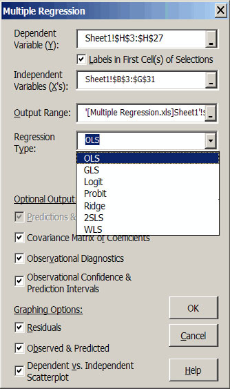Figure 2. Multiple Regression Dialog Box.

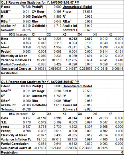
A sample output for a multiple regression in Figure 3 indicates the format for the first part of the results. The name of an X variable and its beta are in bold if the variable is statistically significant at the indicated one minus alpha level (e.g., X1, X2, X3, and X4 in the example). Standard errors for the betas, the t-test statistics and the probability (pr) value of the t-statistics are provided for each explanatory variable. The elasticity at the mean for each independent variable as well as the partial and semi partial correlations for these variables are also provided. The variance inflation factor is reported for each X variable to indicate the degree of multicollinearity of Xi to other variables in the model.

The Restriction row in the parameter block of output values allows the user to interactively experiment with various combinations of X variables. After the initial parameter estimation the Restriction coefficients are all blank (Figure 3), meaning that every X variable is included in the unrestricted model. The user can interactively drop and re-include a variable by changing its restriction coefficient to 0 or blank. Three test statistics (F, R2 and ) for the Unrestricted Model are provided and remain fixed while testing alternative specifications of the model’s variables. This is done to facilitate the comparison to the original unrestricted model to the restricted models. If you type a non-zero number in the restriction row, the value becomes the beta-hat coefficient for a restricted regression.

Figure 3. Sample Output for a Restricted Multiple Regression Model.

In addition to the ability to exclude/re-include variables in the model, Simetar’s multiple regression function allows one to make corrections to the data for the actual observations of the X and Y values, without having to re-run the regression. In addition, the Simetar© multiple regression routine is not limited in the number of exogenous variables observation that can be included in the model.

The covariance matrix for the betas is provided as output for the multiple regression. The beta covariance matrix is used in simulation when the model is assumed to have stochastic betas. The beta covariance matrix is provided when requested as an option in the multiple regression dialog box.

Residuals from the regression are summarized in a table (Figure 4). The residuals for the regression are calculated as for each observation i. The standard error for the mean predicted value (SE mean predicted) is provided for each observation i. In addition the SE of the Predicted values for each observation is provided in column 5 of the output (Figure 4). The SE of the Predicted values is the correct SE for simulating a probabilistic forecast of the multiple regression forecast values, because it is the SE for predicting “an observation.” As indicated in Figure 4, the SE Predicted Values increase as the forecasted period gets longer. Prediction and confidence intervals for the model are provided in the table and graphically for the alpha equal 5 percent level (Figure 5). 

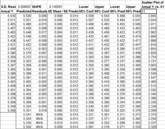Figure 4. Sample Output of Residuals and Confidence and Prediction Intervals for a Multiple Regression.

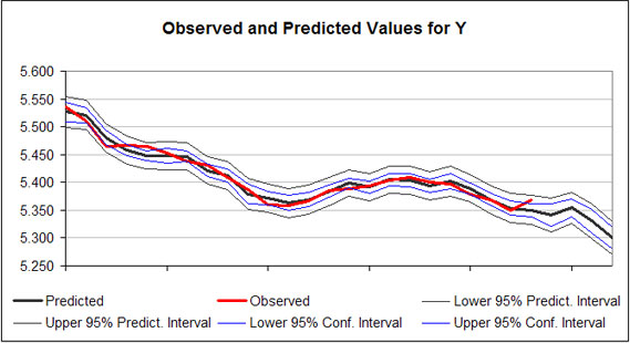Figure 5. Sample Chart of Predicted Regression Results and Prediction Intervals.

Simetar© can calculate (simulate) forecast values for the Y variable (Figure 2) if the associated Xs are provided. For the example in Figure 2, four more rows of X observations are provided than Y observations. The extra X values were used to forecast the Y variable in Figures 4 and 5. The Y forecast values are deterministic simulations of the dependent variable. Confidence intervals and prediction intervals for the regression model are calculated (Figure 4) for each observation, if requested in the dialog box (Figure 2).

If requested in the regression dialog box (Figure 2), observational diagnostics are calculated and reported for the unrestricted model (Figure 6). The column of 1’s in the DFBetas Restriction column indicate that the unrestricted model was fit using all of the observed data. If you change a DFBetas Restriction column indicate that the unrestricted model was fit using all of the observed data. If you change a DFBetas Restriction to 0 for a particular row the model is instantly updated using a dummy variable to ignore the effects for that row of X’s and Y. The rule for excluding an observation is if its Studentized Residual is greater than 2 (is bold). This is the case for observation 24 in the sample output (Figure 6). Setting the Restriction value to 0 for observation 24 causes the F statistic to increase from 88 to 107, given that X6 has not been excluded from the model. The R² increases to 96.9 and R² the increases to 95.8. This result suggests that observation 24 is either an outlier or should be handled with a dummy variable. A priori justification should be used when handling observations in this manner.

A useful feature that the Multiple Regression option has over the Simple Regression is that labels for the X and Y variables can appear in the output. Labels must be included in the first cell of the input area specified for the independent variables and the option for Labels in First Cell of X’s must be specified to see the labels in the output. This is a useful feature if you have several independent variables. See Steps 3 and 4 of DemoSimetar-Est for an example of the Multiple Regression output for Simetar©.

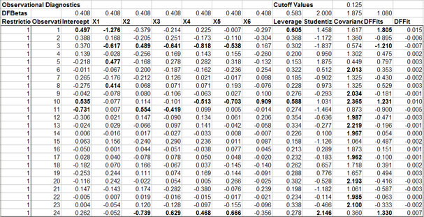Figure 6. Sample Observational Diagnostics for the Multiple Regression.

Probit Analysis. 
The PROBIT function estimates a logistic regression given dependent and independent variables. Probit regression models can be estimated by using the multiple regression Multiple regression icon and selecting the Probit option in the menu, see Figure 2 for the menu. The PROBIT function allows for independent variables to be restricted from the complete model. In addition, individual observations can be restricted from the regression. The PROBIT Function uses an iteratively re-weighted least squares technique to estimate the model parameters. A sample Probit output for Simetar© is presented in Figure 7. 

 Multiple regression 

Figure 7. Sample Probit Output.

Logit Analysis. 
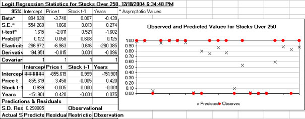
The LOGIT function estimates a logistic regression given dependent and independent variables. Logit regression models can be estimated by using the multiple regression icon Multiple regression and selecting the Logit option in the menu, see Figure 2 for the menu. The LOGIT function allows for independent variables to be restricted from the complete model. In addition, individual observations can be restricted from the regression. The LOGIT Function uses an iteratively re-weighted least squares technique to estimate the model parameters. A sample Logit output for Simetar© is presented in Figure 8.

 Multiple regression 

Figure 8. Sample Logit Output.