Model validation must be done prior to application of the model for decision making. Validation can utilize graphs, such as PDFs and CDFs, but statistical testing of the simulated distributions is required to make sure that the stochastic variables in the model are statistically the same as the historical distributions. To facilitate the validation process several hypothesis tests have been included in Simetar©. The tests are organized using 5 tabs in the Hypothesis Testing for Data dialog box opened by the Statistical tests for validating simulated random variablesicon (Figure 1).
 Statistical tests for validating simulated random variables
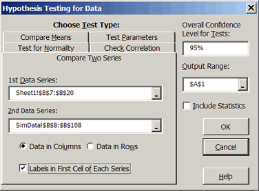 |
| Figure 1. Univariate and Multivariate Distribution Tests. |
The means and variances for two distributions (or series) can be compared by using the Compare Two Series tab for the Hypothesis Testing dialog box opened by the Statistical tests for validating simulated random variables icon. The mean and variance tests are univariate as they only test the values between two variables. This type of hypothesis testing is useful in validation for comparing the simulated distribution to the historical distribution. The test can be repeated for each of the stochastic variables to validate all of the random variables in a model. The means are tested using the Student’s-t test and the variances are tested using the F-test. The null hypotheses are that the simulated mean equals the historical mean and the simulated variance equals the historical variance. The statistical tests are performed when the Compare Two Series tab in Figure 1 is selected and you specify the two distributions (data series) to compare. The two sample Student-t test is used to allow comparison of means from distributions with an un-equal number of observations. See Step 3 in DemoSimetar-Data for an example of comparing two distributions.
Statistical tests for validating simulated random variables
Means and variances for multivariate (MV) probability distributions can be tested against actual data in one step. The MV means test uses the two-sample Hotelling T2 test which tests whether two data matrices (mxn and pxn) have the same mean vectors, assuming normality and equality of covariance matrices of the data matrices. Assume historical data are arranged in an mxn matrix and the simulated data are in a pxn matrix, where p is the number of iterations, then the means can be tested with the Hotelling T2 test procedure. The Hotelling T2 test is analogous to a Student’s-t test of two means in a two-sample univariate case.
The equality of the covariance matrices for two data matrices with dimensions mxn and pxn, respectively, can be tested using a large sample likelihood ratio testing procedure. The Box’s M test of homogeneity of covariances can be used to test whether the covariance matrices of two or more data series, with n columns each, are equal. The assumptions under this test are that the data matrices are MV normal and that the sample is large enough for the asymptotic, or central Chi-Squared, distribution under the null hypothesis to be used.
The third MV test is the Complete Homogeneity test. This statistical test simultaneously tests the mean vectors and the covariance matrices for two distributions. The historical data’s mean vector and covariance matrix are test against the simulated sample’s mean vector and covariance matrix. If the test fails to reject that the means and covariance are equivalent then one can assume that the multivariate distribution in the historical series is being simulated appropriately. An example of this test is provided in Step 4 of DemoSimetar-Data.
The combination of the Hotelling T-Squared test, Box’s M-test, and the Complete Homogeneity test provides an additional tool for validating a multivariate probability distribution. These three MV distribution tests are performed by Simetar© when you specify an mxn matrix for the 1st Data Series and a pxn matrix for the 2nd Data Series after selecting the Compare Two Series tab (Figure 1) for the Hypothesis Testing dialog box opened by the Statistical tests for validating simulated random variables icon. The Compare Two Series tab invokes the MV distribution tests if the 1st and 2nd Data Series indicate two matrices and invokes the univariate student’s-t and F tests if the specified Data Series indicate two different columns.
Statistical tests for validating simulated random variables
Another validation test provided in Simetar© is a test to compare the correlation matrix implicit in the simulated output to the input correlation matrix. This type of test is useful for validating multivariate probability distributions. Selecting the Check Correlation tab in the Hypothesis Testing for Data dialog box (Figure 2) calculates the Student’s-t test statistics for comparing the corresponding correlation coefficients in the two matrices. The dialog box requires information for the location of the simulated series (a pxn matrix) and the location of the original nxn correlation matrix. The confidence level for the resulting Student’s-t test defaults to a value greater than 0.95 but can be changed by the user after the test has been performed. An example of this test is provided in Step 6 of DemoSimetar-Data. If a simulated correlation coefficient is statistically different from the input coefficient, the Student t-test statistic will exceed the Critical Value and its respective Student t-test statistic in the results matrix will be bold.
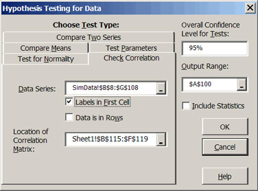 |
| Figure 2. Univariate and Multivariate Distribution Tests. |
The mean and standard deviation for any data series (e.g., simulated data) can be compared to a specified mean and standard deviation using the Test Parameters tab in Figure 3. The Student’s-t test is used to compare the user specified mean to the calculated mean of any distribution (or series) as demonstrated in Figure 3. A Chi-Squared test is used to test a user specified standard deviation to the standard deviation for a simulated distribution. The null hypothesis for both tests is that the statistic for the simulated series equals the user’s specified values. An example of testing a simulated series against a specified mean and standard deviation is provided in Step 5 of DemoSimetar-Data.
|
| Figure 3. Parameter Tests for a Distribution |
Five different tests for normality can be performed by selecting the Test for Normality tab after the Statistical tests for validating simulated random variables icon is selected (Figure 3). The normality tests are: Kolmogornov-Smirnoff, Chi-Squared, Cramer-von Mises, Anderson-Darling, and Shapiro-Wilks. The Chi-Squared test requires the number of bins (or intervals); 20 or more intervals appears to work for most data series. In addition to the normality tests this option calculates the skewness and kurtosis, relative to a normal distribution. See Step 2 in DemoSimetar-Data for an example.
Statistical tests for validating simulated random variables
A measure to compare the difference between two cumulative distribution functions (CDFs) is calculated by the =CDFDEV( ) function. The function calculates the sum of the squared differences between two CDFs with an added penalty for differences in the tails. The scalar is calculated for two CDFs, F(x) and G(x) as:

where: wi is a penalty function that applies more weight to deviations in the tails than values around the mean.
If the G(x) distribution is the same as the F(x) distribution, then the value equals zero. The CDFDEV measure is programmed to compare a historical series (CDF) to a simulated series (CDF) as follows:
=CDFDEV(Range for Historical Series, Range for Simulated Series)
where: Range for Historical Series is the location for the values to define the original or historical data, such as B1:B10, and Range for Simulated Series is the location for the simulated values, such as B9:B109. The number of values for the two series does not have to be equal.
The =CDFDEV( ) function is most useful when testing the ability of different assumed probability distributions to simulate a random variable. In this case, the CDFDEV measure is calculated using the simulated values for each of the alternative probability distributions. The probability distribution associated with the lowest CDFDEV scalar is the “best” distribution for simulating the random variable. For an example see Step 9 in DemoSimetar-Est for a demonstration of using =CDFDEV( ) to compare alternative distributions for simulating a random variable.